Sensitivity to Unobserved Confounding in Studies with Factor-structured Outcomes
9/28/23
Slides and Paper
Slides: afranks.com/talks
Sensitivity to Unobserved Confounding in Studies with Factor-structured Outcomes, (JASA, 2023) https://arxiv.org/abs/2208.06552
Joint work with Jiajing Zheng (formerly UCSB), Jiaxi Wu (UCSB) and Alex D’Amour (Google)
Causal Inference From Observational Data
Consider a treatment \(T\) and outcome \(Y\)
Interested in the population average treatment effect (PATE) of \(T\) on \(Y\): \[E[Y | do(T=t)] - E[Y | do(T=t')]\]
- In general, the PATE is not the same as \[E[Y | T=t] - E[Y | T=t']\]
Confounders
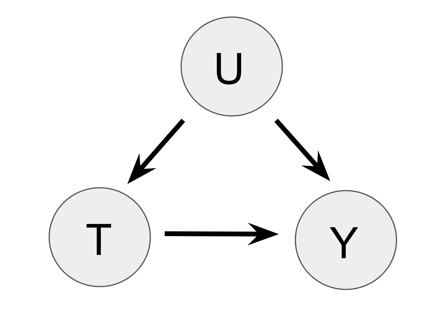
Confounding bias
- Observed data regression of \(T\) on \(Y\) fails because the distribution of \(U\) varies in the two treatment arms
- We try to condition on as many observed confounders as possible to mitigate potential confounding bias
- Commonly assumed that there are “no unobserved confounders” (NUC) but this is unverifiable
- Sensitivity analysis is a tool for assessing the impacts of violations of this assumption
A Motivating Example

A Motivating Example

The Effects of Light Alcohol Consumption
Observational data from the National Health and Nutrition Examination Study (NHANES) on alcohol consumption.
Light alcohol consumption is positively correlated with blood levels of HDL (“good cholesterol”)
Define “light alcohol consumption’’ as 1-2 alcoholic beverages per day
Non-drinkers: self-reported drinking of one drink a week or less
Control for age, gender and indicator for educational attainment
HDL and alcohol consumption
Call:
lm(formula = Y[, "HDL"] ~ drinking + X)

Residuals:
    Min      1Q  Median      3Q     Max
-5.0855 -0.6127 -0.0512  0.6389  4.2383

Coefficients:
            Estimate Std. Error t value Pr(>|t|)
(Intercept) 0.225550   0.091105   2.476 0.013412 *
drinking    0.597399   0.091917   6.499 1.11e-10 ***
Xage        0.006409   0.001452   4.415 1.09e-05 ***
Xgender     0.689557   0.049426  13.951  < 2e-16 ***
Xeduc       0.194338   0.051161   3.799 0.000152 ***
---
Signif. codes:  0 '***' 0.001 '**' 0.01 '*' 0.05 '.' 0.1 ' ' 1

Residual standard error: 0.9216 on 1434 degrees of freedom
Multiple R-squared:  0.1531,    Adjusted R-squared:  0.1507
F-statistic: 64.81 on 4 and 1434 DF, p-value: < 2.2e-16Blood mercury and alcohol consumption
Call:
lm(formula = Y[, "Methylmercury"] ~ drinking + X)

Residuals:
    Min      1Q  Median      3Q     Max
-2.3570 -0.7363 -0.0728  0.6242  4.1127

Coefficients:
             Estimate Std. Error t value Pr(>|t|)
(Intercept)  0.442044   0.096385   4.586 4.91e-06 ***
drinking     0.364096   0.097244   3.744 0.000188 ***
Xage         0.008186   0.001536   5.330 1.14e-07 ***
Xgender     -0.062664   0.052290  -1.198 0.230966
Xeduc        0.269815   0.054126   4.985 6.95e-07 ***
---
Signif. codes:  0 '***' 0.001 '**' 0.01 '*' 0.05 '.' 0.1 ' ' 1

Residual standard error: 0.975 on 1434 degrees of freedom
Multiple R-squared:  0.05209,   Adjusted R-squared:  0.04945
F-statistic: 19.7 on 4 and 1434 DF, p-value: 8.41e-16Residual Correlation
    Pearson's product-moment correlation

data:  hdl_fit$residuals and mercury_fit$residuals
t = 3.7569, df = 1437, p-value = 0.0001789
alternative hypothesis: true correlation is not equal to 0
95 percent confidence interval:
 0.04718758 0.14953581
sample estimates:
      cor
0.0986225
Residual correlation might be indicative of confounding bias
Sensitivity Analysis
NUC unlikely to hold exactly. What then?
Calibrate assumptions about confounding to explore range of causal effects that are plausible
Robustness: quantify how “strong” confounding has to be to nullify causal effect estimates
- Well established methods for single outcome analyses
Multi-outcome Sensitivity Analysis
- If we measure multiple outcomes, is there prior knowledge that we can leverage to strengthen causal conclusions?
- What might residual correlation in multi-outcome models mean for potential for confounding?
How do results change when we assume a priori that certain outcomes cannot be affected by treatments?
- Null control outcomes (e.g. alcohol consumption should not increase mercury levels)
Standard Assumptions
Assumption (Latent Ignorability)
U and X block all backdoor paths between T and Y (Pearl 2009)
Assumption (Latent positivity)
f(T = t | U = u, X = x) > 0 for all u and x
Assumption (SUTVA)
There are no hidden versions of the treatment and there is no interference between units
Single-outcome Sensitivity Analysis
Result (Cinelli and Hazlett 2020)
Assume the outcome is linear in the treatment and confounders (no interactions). Then the squared omitted variable bias for the PATE is \[\text{Bias}_{t_1,t_2}^2 \, \leq \, \frac{(t_1-t_2)^2}{\sigma_{t\mid x}^2} \left(\frac{R^2_{T\sim U|X}}{1 - R^2_{T\sim U|X}} \right)R^2_{Y \sim U | T, X}\]
Single-outcome Sensitivity Analysis
Result (Cinelli and Hazlett 2020)
Assume the outcome is linear in the treatment and confounders (no interactions). Then the squared omitted variable bias for the PATE is \[\text{Bias}_{t_1,t_2}^2 \, \leq \, \frac{(t_1-t_2)^2}{\sigma_{t\mid x}^2} {\color{#C43424}\left(\frac{R^2_{T\sim U|X}}{1 - R^2_{T\sim U|X}} \right)}R^2_{Y \sim U | T, X}\]
- \(R^2_{T\sim U|X}\): partial fraction of treatment variance explained by confounders (given observed covariates)
Single-outcome Sensitivity Analysis
Result (Cinelli and Hazlett 2020)
Assume the outcome is linear in the treatment and confounders (no interactions). Then the squared omitted variable bias for the PATE is \[\text{Bias}_{t_1,t_2}^2 \, \leq \, \frac{(t_1-t_2)^2}{\sigma_{t\mid x}^2} \left(\frac{R^2_{T\sim U|X}}{1 - R^2_{T\sim U|X}} \right){\color{#C43424}R^2_{Y \sim U | T, X}}\]
\(R^2_{T\sim U|X}\): partial fraction of treatment variance explained by confounders (given observed covariates)
\(R^2_{Y\sim U|T,X}\): partial fraction of outcome variance explained by confounders (given observed covariates and treatment)
Robustness
- How big do \(R^2_{T\sim U |X}\) and \(R^2_{Y \sim U | T, X}\) need to be to nullify the effect?
- \(RV^1\) smallest value of \(R^2_{T\sim U |X} = R^2_{Y \sim U | T, X}\) needed to nullify effect (Cinelli and Hazlett 2020)
- \(XRV\) smallest value of \(R^2_{T\sim U |X}\) assuming \(R^2_{Y \sim U | T, X}=1\) needed to nullify effect (Cinelli and Hazlett 2022)
Calibrating Sensitivity Parameters
What values of \(R^2_{Y\sim U|T, X}\) and \(R^2_{T \sim U | X}\) might be reasonable?
Can use observed covariates to generate benchmark values:
Compute \(R^2_{T \sim X_{j} | X_{-j}}\) for all covariate \(X_j\)
Compute \(R^2_{Y \sim X_{j} | X_{-j}, T}\) for all covariate \(X_j\)
Use domain knowledge to reason about most important confounders
Sensitivity of HDL Cholesterol Effect
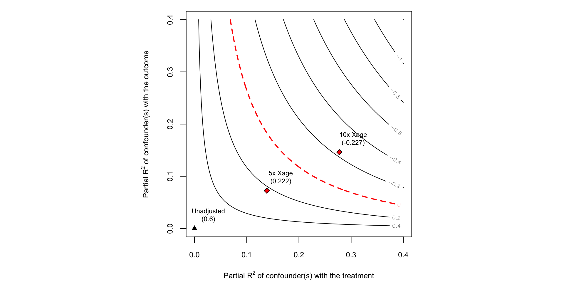
From the sensemakr documentation (Cinelli, Ferwerda, and Hazlett 2020)
Models with factor-structured residuals
Assume the observed data mean and covariance can be expressed as follows: \[\begin{align}
E[Y \mid T = t, X=x] &= \check g(t, x)\\
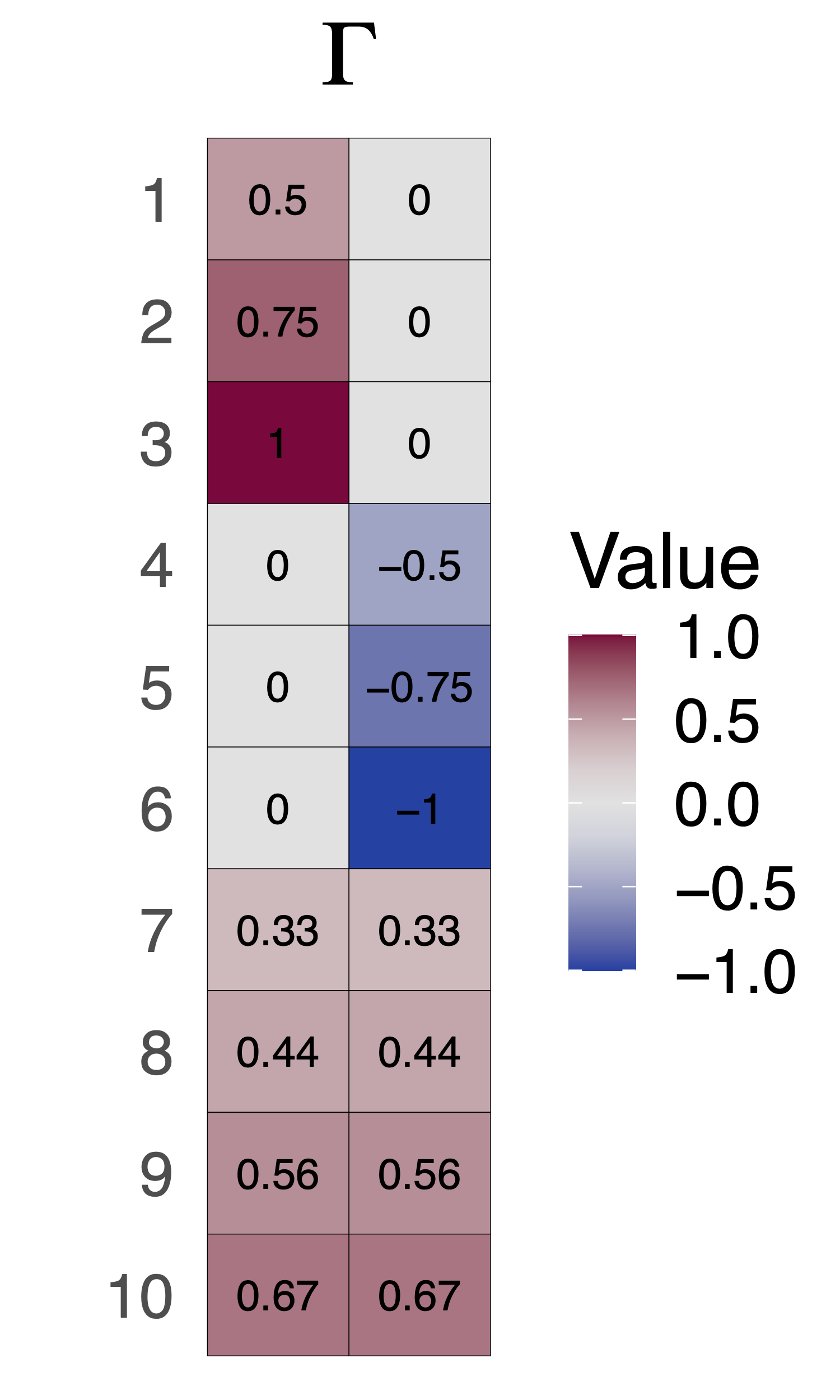
Cov(Y \mid T = t, X = x) &= \Gamma\Gamma' + \Lambda,
\end{align}\]
- \(\Gamma\) are factor loading matrices, \(\Lambda\) is diagonal
- \(\check g(T=t, X) - \check g(T=t', X)\) is only the PATE when there is NUC
A Structural Equation Model
\(U\) (m-vector) and \(X\) are possible causes for \(T\) (scalar) and \(Y\) (q-vector)
\(X\) are observed but \(U\) are not.
\[\begin{align} & U = \epsilon_U \label{eqn:u}\\ &T = f_{\epsilon}(X, U) \label{eqn:treatment_general,multi-y}\\ &Y = g(T,X) + \Gamma\Sigma_{u|t,x}^{-1/2}U + \epsilon_{y}, \label{eqn:epsilon_y} \end{align}\]
- This SEM is compatible the factor structured residuals, \(Cov(Y|T, X) = \Gamma\Gamma' + \Lambda\)
A Structural Equation Model
\[\begin{align} &U = \epsilon_U\\ &T = f_\epsilon(X,U)\\ &Y = g(T, X) + \Gamma\Sigma_{u|t,x}^{-1/2}U + \epsilon_{y} \end{align}\]
Confounding bias is \(\Gamma\Sigma_{u|t,x}^{-1/2}\mu_{u \mid t,x}\)
\(\mu_{u \mid t,x}\) and \(\Sigma_{u|t,x}\) are the conditional mean and covariance of the unmeasured confounders
- User specified sensitivity parameters
A Sensitivity Specification
- Interpretable specification for \(\mu_{u \mid t,x}\) and \(\Sigma_{u|t,x}\) parameterized by a single \(m\)-vector, \(\rho\):
\[\begin{align} \mu_{u\mid t,x} &= \frac{\rho}{\sigma_{t \mid x}^{2}}\left(t-\mu_{t\mid x}\right) \label{eqn:conditional_u_mean}, \\ \Sigma_{u \mid t,x} &= I_m-\frac{\rho \rho^{\prime}}{\sigma_{t\mid x}^{2}} \label{eqn:conditional_u_cov}, \end{align}\]
\(\rho\) is the partial correlation vector between \(T\) and \(U\)
Define \(0 \leq R^2_{T \sim U |X}:= \frac{||\rho||^2_2}{\sigma^2_{t\mid x}} < 1\) to be the squared norm of the partial correlation between T and U given \(X\)
Multi-Outcome Assumptions
Assumption (Homoscedasticity)
\(Cov(Y |T = t, X = x)\) is invariant to t and x. Implies factor loadings, \(\Gamma\), are invariant to \(t\) and \(x\)
Assumption (Factor confounding)
The factor loadings, \(\Gamma\), are identifiable (up to rotation) and reflect all potential confounders. (Anderson and Rubin 1956)
To identify factor loadings, \(\Gamma\), \((q-m)^2-q-m\geq0\) and each confounder must influence at least three outcomes
Bounding the Omitted Variable Bias
Theorem (Bounding the bias for outcome \(Y_j\))
Given the structural equation model, sensitivity specification and given assumptions, the squared omitted variable bias for the PATE of outcome \(Y_j\) is bounded by \[\text{Bias}_{j}^2 \, \leq \, \frac{(t_1-t_2)^2}{\sigma_{t\mid x}^2} \left(\frac{R^2_{T\sim U|X}}{1 - R^2_{T\sim U|X}} \right)\parallel \Gamma_j\parallel_2^2\]
The bound on the bias for outcome \(j\) is proportional to the norm of the factor loadings for that outcome
A single sensitivity parameter, \(R^2_{T \sim U \mid X}\), shared across all outcomes
Bounding the Omitted Variable Bias
Theorem (Bounding the bias for outcome \(Y_j\))
Given the structural equation model, sensitivity specification and given assumptions, the squared omitted variable bias for the PATE of outcome \(Y_j\) is bounded by \[\text{Bias}_{j}^2 \, \leq \, \frac{(t_1-t_2)^2}{\sigma_{t\mid x}^2} \left(\frac{R^2_{T\sim U|X}}{1 - R^2_{T\sim U|X}} \right){\color{#C43424} \parallel \Gamma_j\parallel_2^2}\]
The bound on the bias for outcome \(j\) is proportional to the norm of the factor loadings for that outcome
A single sensitivity parameter, \(R^2_{T \sim U \mid X}\), shared across all outcomes
Bounding the Omitted Variable Bias
Theorem (Bounding the bias for outcome \(Y_j\))
Given the structural equation model, sensitivity specification and given assumptions, the squared omitted variable bias for the PATE of outcome \(Y_j\) is bounded by \[\text{Bias}_{j}^2 \, \leq \, \frac{(t_1-t_2)^2}{\sigma_{t\mid x}^2} {\color{#C43424}\left(\frac{R^2_{T\sim U|X}}{1 - R^2_{T\sim U|X}} \right)} \parallel \Gamma_j\parallel_2^2\]
The bound on the bias for outcome \(j\) is proportional to the norm of the factor loadings for that outcome
A single sensitivity parameter, \(R^2_{T \sim U \mid X}\), shared across all outcomes
Reparametrizing \(R^2_{T \sim U | X}\) for binary treatments
\(R^2_{T \sim U | X}\) is unnatural for binary treatments
\(\Lambda\)-parameterization \(\leftrightarrow\) \(R^2_{T \sim U | X}\)-parameterization
Fix a \(\Lambda_\alpha\) such that \[Pr\left(\Lambda_\alpha^{-1} \leq \frac{e_0(X, U)/(1-e_0(X, U))}{e(X)/(1-e(X))}\leq \Lambda_\alpha\right)=1-\alpha\]
- Related to the marginal sensitivity model (Tan 2006)
Null Control Outcomes
- Assume we have null control outcomes, \(\mathcal{C}\)
- \(\check \tau\) are the vector of PATEs under NUC
- \(\Gamma_{\mathcal{C}}\) are the factor loadings for the null control outcomes, \(\mathcal{C}\)
- Need at least \(R^2_{T \sim U \mid X}\geq R^2_{min}\) of the treatment variance to be due to confounding to nullify the null controls
Null Control Outcomes
Theorem (Bias with Null Control Outcomes)
Assume the previous structural equation model and sensitivity specification. Then the squared omitted variable bias for the PATE of outcome \(Y_j\) is bounded by
\[\begin{equation} \label{eqn:ignorance-region-gaussian-wnc,multi-y} \text{Bias}_j \in \left[\Gamma_j \Gamma_{\mathcal{C}}^{\dagger} \check{\tau}_{\mathcal{C}} \; \pm \; \parallel \Gamma_j P_{\Gamma_{\mathcal{C}}}^{\perp} \parallel_2 \sqrt{ \frac{1}{\sigma_{t\mid x}^2}\left( \frac{R^2_{T \sim U | X}}{1 - R^2_{T \sim U | X}} - \frac{R^2_{min}}{1 - R^2_{min}} \right)} \right], \end{equation}\]
Null Control Outcomes
Theorem (Bias with Null Control Outcomes)
Assume the previous structural equation model and sensitivity specification. Then the squared omitted variable bias for the PATE of outcome \(Y_j\) is bounded by
\[\begin{equation} \text{Bias}_j \in \left[{\color{#C43424}\Gamma_j \Gamma_{\mathcal{C}}^{\dagger} \check{\tau}_{\mathcal{C}}} \; \pm \; \parallel \Gamma_j P_{\Gamma_{\mathcal{C}}}^{\perp} \parallel_2 \sqrt{ \frac{1}{\sigma_{t\mid x}^2}\left( \frac{R^2_{T \sim U | X}}{1 - R^2_{T \sim U | X}} - \frac{R^2_{min}}{1 - R^2_{min}} \right)} \right], \end{equation}\]
- \(\Gamma_j\Gamma_{\mathcal{C}}^{\dagger}\check \tau_{\mathcal{C}}\) is a (partial) bias correction for outcome \(j\)
Null Control Outcomes
Theorem (Bias with Null Control Outcomes)
Assume the previous structural equation model and sensitivity specification. Then the squared omitted variable bias for the PATE of outcome \(Y_j\) is bounded by
\[\begin{equation} \text{Bias}_j \in \left[\Gamma_j \Gamma_{\mathcal{C}}^{\dagger} \check{\tau}_{\mathcal{C}} \; \pm \; \parallel \Gamma_j P_{\Gamma_{\mathcal{C}}}^{\perp} \parallel_2 \sqrt{ \frac{1}{\sigma_{t\mid x}^2}\color{#C43424}{\left( \frac{R^2_{T \sim U | X}}{1 - R^2_{T \sim U | X}} - \frac{R^2_{min}}{1 - R^2_{min}} \right)}} \right], \end{equation}\]
- If \(R^2_{T \sim U | X}=R^2_{min}\) then the bias is identified for all outcomes
Null Control Outcomes
Theorem (Bias with Null Control Outcomes)
Assume the previous structural equation model and sensitivity specification. Then the squared omitted variable bias for the PATE of outcome \(Y_j\) is bounded by
\[\begin{equation} \text{Bias}_j \in \left[\Gamma_j \Gamma_{\mathcal{C}}^{\dagger} \check{\tau}_{\mathcal{C}} \; \pm \; {\color{#C43424}\parallel \Gamma_j P_{\Gamma_{\mathcal{C}}}^{\perp} \parallel_2} \sqrt{ \frac{1}{\sigma_{t\mid x}^2}\left( \frac{R^2_{T \sim U | X}}{1 - R^2_{T \sim U | X}} - \frac{R^2_{min}}{1 - R^2_{min}} \right)} \right], \end{equation}\]
- Ignorance about the bias is smallest when \(\Gamma_j\) is close to the span of \(\Gamma_{\mathcal{C}}\), that is, when \(\parallel \Gamma_j P_{\Gamma_{\mathcal{C}}}^{\perp} \parallel_2\) is small
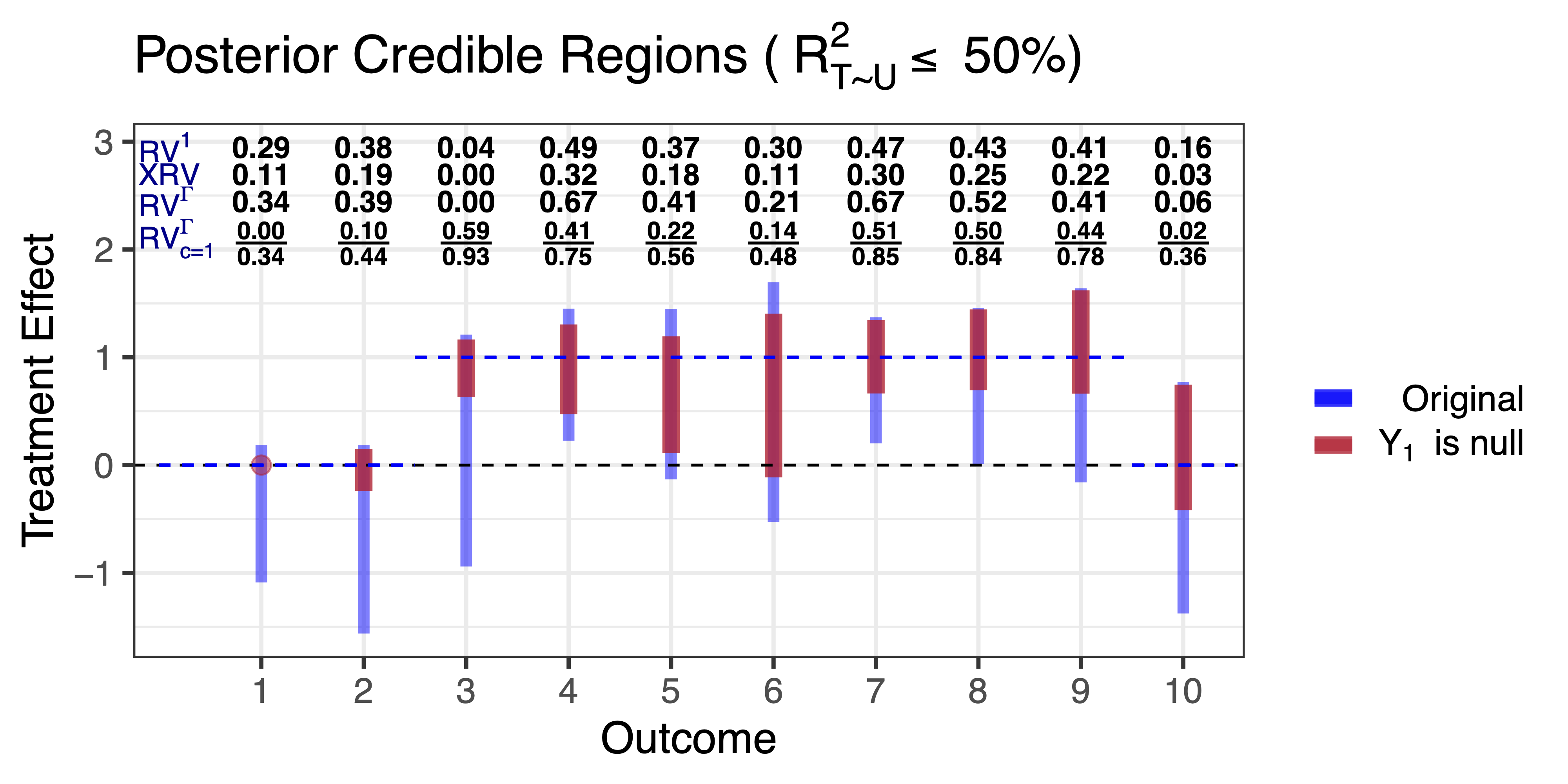
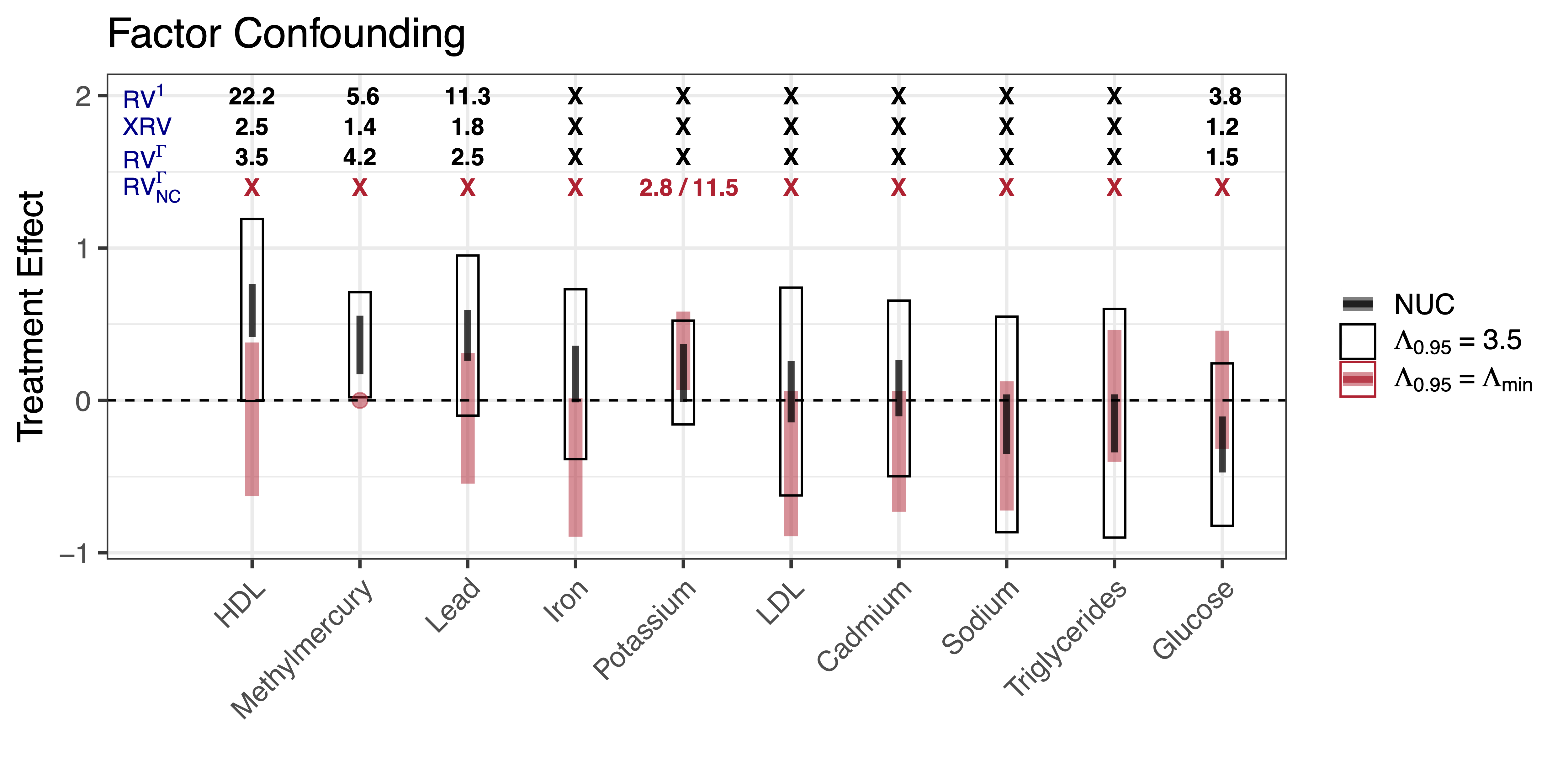
Robustness under Factor Confounding
- \(RV^\Gamma_j\) smallest value of \(R^2_{T\sim U |X}\) needed to nullify the effect for outcome \(j\) under factor confounding
\(RV^\Gamma_j\) can be smaller or larger than \(RV^1\)
\(RV_j^{\Gamma} \geq XRV\) by definition
- \(RV^\Gamma_{j, NC}\) smallest value of \(R^2_{T\sim U |X}\) needed to nullify the effect for outcome \(j\) and the assumed null controls
Simulation Study
Gaussian data generating process \[\begin{align} T &= \beta' U + \epsilon_T \\ Y_j &= \tau_jT + \Gamma'\Sigma^{-1/2}_{u|t}U + \epsilon_y \end{align}\]
\(R^2_{T \sim U \mid X}=0.5\) from \(m=2\) unmeasured confounders
\(\tau_j = 0\) for \(Y_1\), \(Y_2\) and \(Y_{10}\)
\(\tau_j=1\) for all outher outcomes
Simulation Study
Fit a Bayesian linear regression on the 10 outcomes given then treatment
Assume a residual covariance with a rank-two factor structure
Plot ignorance regions assuming \(R^2_{T \sim U} \leq 0.5\)
Plot ignorance regions assuming \(R^2_{T \sim U} \leq 0.5\) and \(Y_1\) is null
Simulation Study
The effects of light drinking
- Measure ten different outcomes from blood samples:
- natural: HDL, LDL, triglycerides, potassium, iron, sodium, glucose
- environmental toxicants: mercury, lead, cadmium.
- Measured confounders: age, gender and indicator for highest educational attainment
- Residual correlation in the outcomes might be indicative of additional confounding bias
The effects of light drinking
Model: \[\begin{align} Y &\sim N(\tau T + \alpha 'X, \Gamma\Gamma' + \Lambda) \end{align}\]
\(E[Y| T, X, U] = \tau T + \alpha 'X + \Gamma'\Sigma^{-1/2}_{u|t}U\)
Residuals are approximately Gaussian
Fit a multivariate Bayesian linear regression with factor structured residuals on all outcomes
- Need to choose rank of \(\Gamma\), we use PSIS-LOO (vehtari2017practical?)
- Consider posterior distribution of \(\tau\) under different assumptions about \(R^2_{T\sim U|X}\) and null controls
Benchmark Values
Use age, gender and an indicator of educational attainment to benchmark
\(\frac{1}{3.5} \leq \text{Odds}(X)/\text{Odds}(X_{-age}) \leq 3.5\) for 95% of observed values
For gender and education indicators the odds change was between \(\frac{1}{1.5}\) and \(1.5\)
Assume light drinking has no effect on methylmercury levels
Results: NHANES alcohol study
![]()
Takeaways
Prior knowledge unique to the multi-outcome setting can help inform assumptions about confounding
Sharper sensitivity analysis, when assumptions hold
Negative control assumptions can potentially provide strong evidence for or against robustness
Future directions
- Identification with multiple treatments multiple outcomes
- Collaboration on effects of pollutants on multiple heath outcomes
- Sensitivity analysis for more general models / forms of dependence.
References
Thanks!


Jiaxi Wu (top, UCSB)
Jiajing Zheng (middle, formerly UCSB)
Alex D’Amour (bottom, Google Research)
Sensitivity to Unobserved Confounding in Studies with Factor-structured Outcomes https://arxiv.org/abs/2208.06552