Quantifying Heterogeneity in the Causal Impact of Abortion Restrictions

Alexander Franks

UC Santa Barbara

2025-04-23

Research Team

Elizabeth Stuart
Statistician, Hopkins

Avi Feller
Statistician, UC Berkeley

Alison Gemill
Demographer, Hopkins

Suzanne Bell
Demographer, Hopkins

David Arbour
Statistician, Adobe

Eli Ben-Michael
Statistician, Carnegie Mellon

Texas Senate Bill 8
Effectively bans abortion
Sept. 1, 2021

Roe v. Wade overturned
June 24, 2022

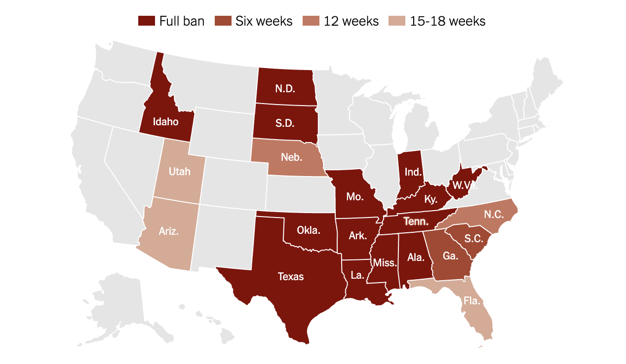
Abortion Bans Across the US

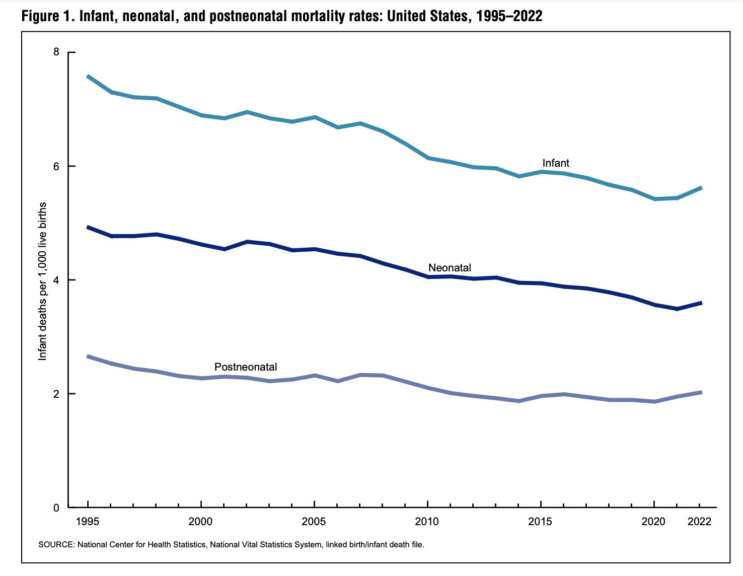
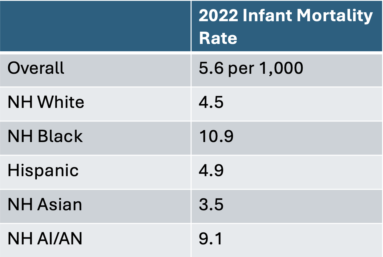
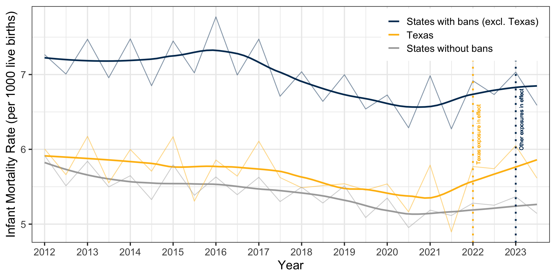
US Infant Mortality Rates

Source: Washington Post, August 18, 2022

Early Evidence on Impacts

• States with abortion bans experienced an average 2.3% increase in births in first half of 2023 (Dench, Pineda-Torres, and Myers 2024)

• By race/ethnicity: greater impact among non-Hispanic Black and Hispanic individuals (Dench, Pineda-Torres, and Myers 2024; Caraher 2024) and greater impact among 20-24-year-olds (Dench, Pineda-Torres, and Myers 2024)

• ~13% increase in infant deaths; 8% increase in the infant mortality rate (Gemmill et al. 2024)

Study Objectives

• To estimate sociodemographic variation in the impact of abortion bans on subnational birth rates in the US through the end of 2023

  • By age, race/ethnicity, marital status, educational attainment, insurance type

• To estimate variation in the impact of abortion bans on subnational infant mortality in the US through the end of 2023
  • By race/ethnicity, timing of death, cause of death

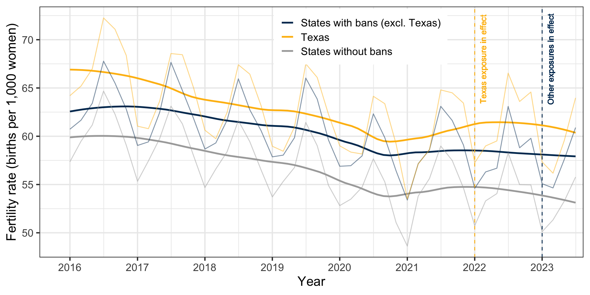
Fertility Trends

Infant Mortality Trends

Overall Analytic Approach

• Today: focus methods discussion on infant mortality data
• Models for the fertility data are very similar
• Bayesian panel data approach

• Poisson latent factor model
  • Fertility: model bimonthly number of births with population offset
  • Infant mortality: model biannual number of deaths with live birth offset
• Model state-by-subgroup-specific impacts separately by characteristic
• States without bans and pre-exposure outcomes in all states inform counterfactual

Infant Mortality Approach

• Outcome: infant mortality rate (deaths per 1,000 live births)
• Exposure: 6-week or complete abortion ban (14 states¹), staggered adoption
• Pre-policy period: January 2012 through ~December 2022
• Treated period: ~January 2023 through December 2023

• Subgroups
  • Race/ethnicity: non-Hispanic White, non-Hispanic Black, Hispanic, and Other
  • Timing: neonatal (<28 days), non-neonatal
  • Cause of death: congenital, non-congenital

1. *States include Alabama, Arkansas, Georgia, Idaho, Kentucky, Louisiana, Mississippi, Missouri, Oklahoma, South Dakota, Tennessee, Texas, West Virginia, Wisconsin

Panel Data

• Panel with \(n\) states and \(T\) time periods
• Potential outcomes \(Y_{it}(0)\), \(Y_{it}(1)\) and a binary exposure indicator \(W_{it} \in \{0,1\}\)
• We observe for each unit the pair \(Y_i, W_i\) where \(Y_{it} \equiv Y_{it}(W_{it}) = \begin{cases} Y_{it}(0) & \text{if } W_{it} = 0\\ Y_{it}(1) & \text{if } W_{it} = 1 \end{cases}\)

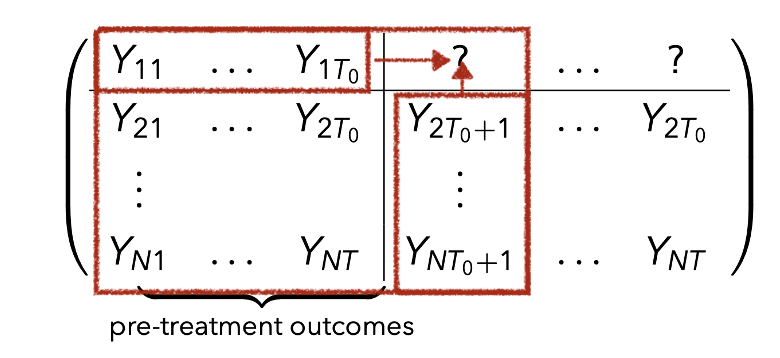
Causal Inference for Panel Data

Assumptions:

• Well-defined exposure: {any complete or 6-week abortion ban} vs {no ban}

• No anticipation: no effect of abortion restrictions prior to exposure

• No spillovers across states: outcomes only depend on own state’s policy

Causal Inference for Panel Data

Some common strategies:

• Interrupted Time Series (horizontal)
• Synthetic Control Methods and Factor Models (vertical)
• Differences in Differences(DID) and Two-Way-Fixed-Effects (TWFE)

Challenges with Infant Death Data

• Infant death counts are small and discrete
• Missing data: CDC Wonder excludes counts between 1 and 9
  • Implications for level of temporal aggregation
• States and subgroups vary in size and mortality rates
• Staggered Adoptions
  • Bans were imposed at different times

Temporal Aggregation

• Missingness → CDC Wonder suppresses counts 1, …, 9 (but not 0!)
  • e.g., annual → no missingness; daily → high missingness
  • Later: imputation approach
• Noise → noise for (avg) annual counts ≪ (avg) monthly counts (see Sun, Ben-Michael, and Feller 2024)
  • Further complicated by seasonality
• Fertility → 2 month intervals (e.g., Jan-Feb 2023)
• Mortality → 6 month intervals (e.g., Jan-June 2023)

Subgroup Inference

• Summing infant deaths over subroups yields total infant deaths

• Inferred total infant mortality rates by differ depending on which subgroups are considered

• Better to estimate the total effect by estimating the subgroup effects and summing or modeling the total effect directly?

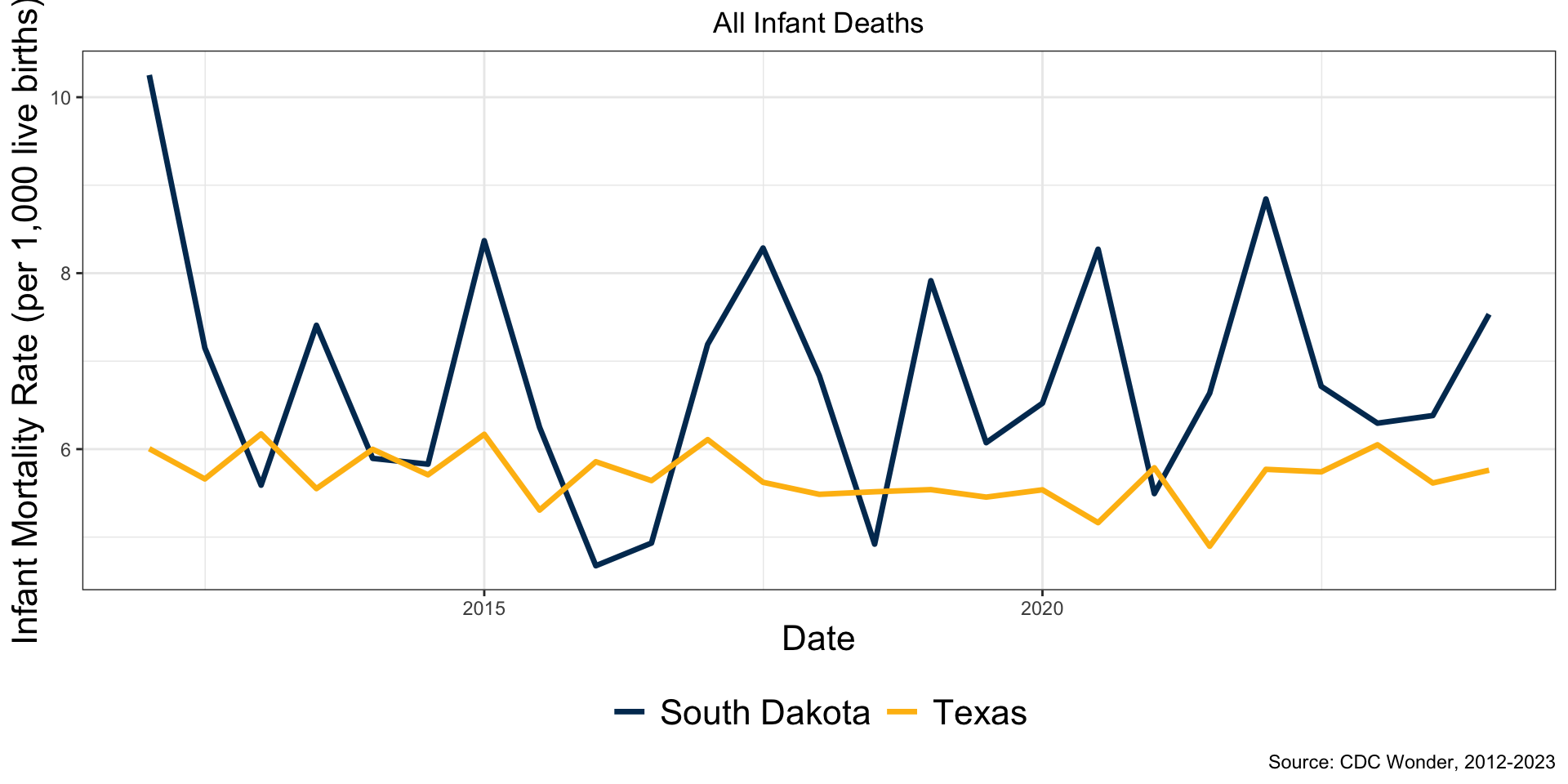
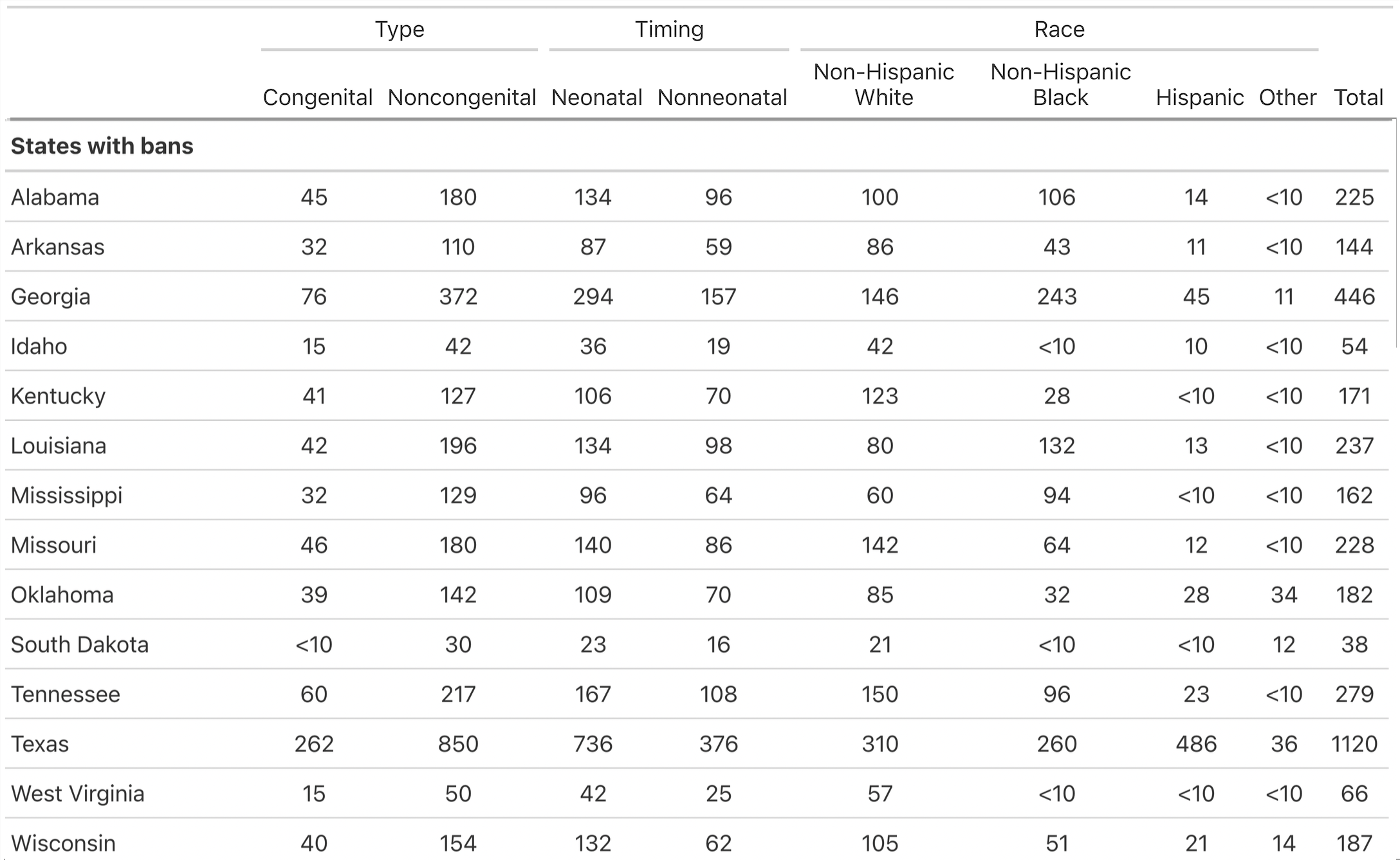
State Size and Sampling Variance

Subgroup Size and Variability

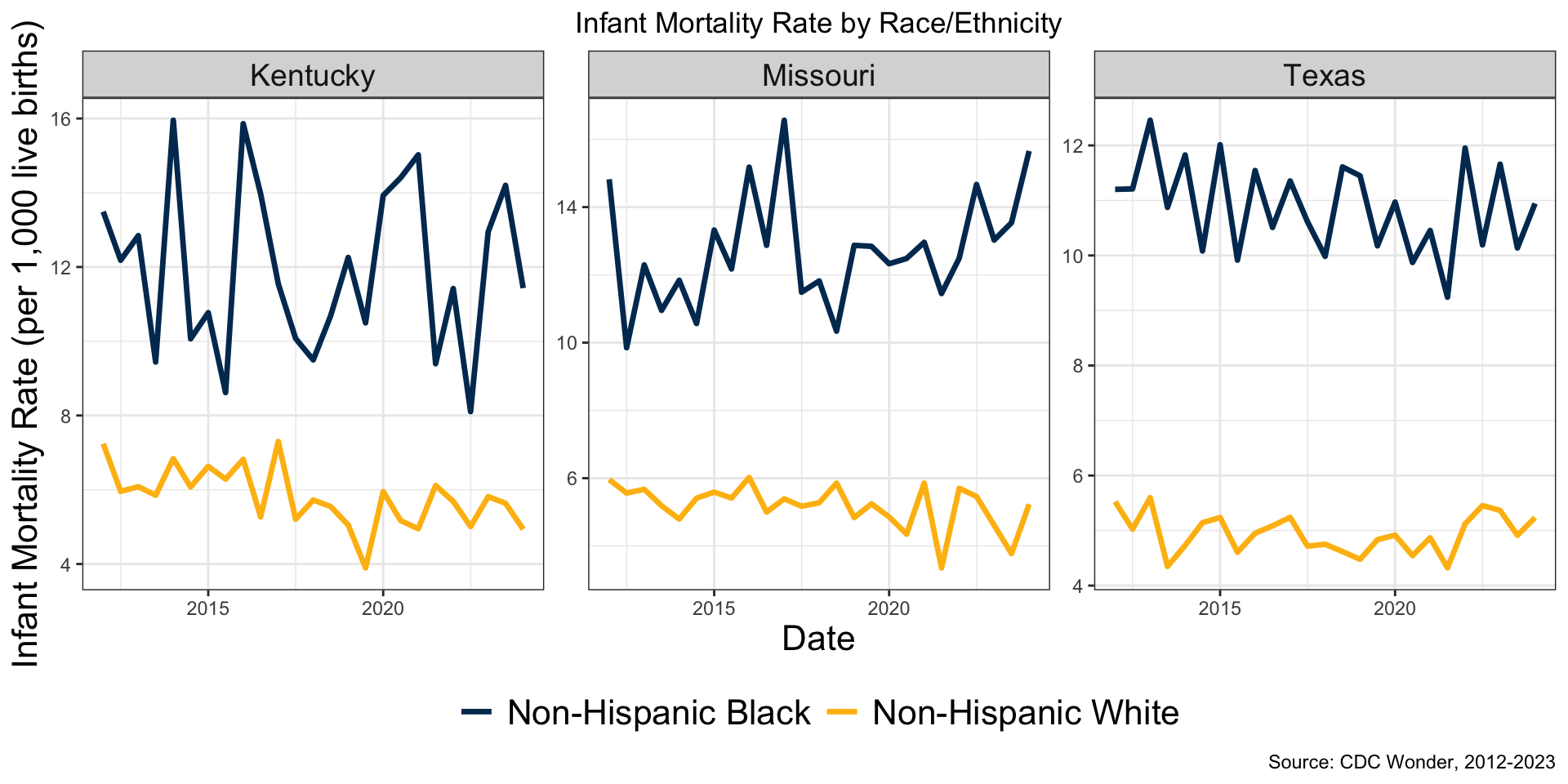
In these states population white ≈ 5-15x population black

Implications

• Pre-treatment balance should depend on state and subgroup size

• Avoid overfitting to noise when groups are small

• The difference between realized and counterfactual infant deaths, \(Y_{it}(1) - Y_{it}(0)\), will be more variable for smaller states and subgroups

• Suggests a need to regularize causal effect estimates

• Want to encourage estimated infant mortality rates to be similar for the same state or same subgroup, while still allowing for the possibility of differences

A Probabilistic Bayesian Model

• Explicitly incorporate a missing data model
• Staggered adoption accounted for in the likelihood
• Count data modeled via Poisson with offset based on state/group size
• Hierarchical prior stabilize treatment effect estimates and partially pool effects by state and category
• Uncertainty quantification for “free”

Panel Model for Infant Deaths

\[ \begin{align} Y_{ijt}(1) &\sim \text{Poisson}(\tau_{ijt} \cdot \rho_{ijt} \cdot B_{ijt})\\ Y_{ijt}(0) &\sim \text{Poisson}(\rho_{ijt} \cdot B_{ijt}) \end{align} \] for unit \(i\), subgroup \(j\), time \(t\)

• \(B_{ijt}\) is births (in thousands)
  • Scales mortality rate to account for variability in state size
• \(\rho_{ijt}\) is the infant mortality rate without bans
• \(\tau_{ijt}\rho_{ijt}\) is the infant mortality rate with bans
• \(\tau_{ijt}\) is the multiplicate change in infant mortality rate due to bans

Poisson Latent Factor Model

We assume the infant mortality rate in the “no ban” condition can be expressed as

\[\rho_{ijt} = \alpha_{ij}^{\text{state}} \cdot \alpha_{jt}^{\text{time}} \cdot \left(\sum_{k=1}^K \lambda_{ijk}\eta_{jkt}\right),\]

• \(\alpha_{ij}^{\text{state}}\) and \(\alpha_{jt}^{\text{time}}\) are state and time-specific intercept
• \(\eta_{jkt} \in \mathbb{R}^+\) is the \(k\)th latent factor at time t, common to all states but unique to subcategory j
• \(\lambda_{ij.} \sim \text{Dirichlet}\) are the factor loadings for state i and category j
• Model selection problem: choosing \(K\) (rank)

Hierarchical Prior on Causal Effects

Partially pool the exposure parameters \(\tau_{ijt}\) across states and across subcategories, with state and subcategory prior distributions centered at zero:

\[ \begin{align} \log(\tau_{ijt}) &\sim N\left(\beta_{ij}^{\text{state,sub}}, \sigma_\tau\right)\\ \beta_{ij}^{\text{state,sub}} &\sim N\left(\beta_i^{\text{state}} + \beta_j^{\text{sub}}, \sigma_\beta\right)\\ \beta_i^{\text{state}} &\sim N\left(0, \sigma_{\text{state}}\right)\\ \beta_j^{\text{sub}} &\sim N\left(0, \sigma_{\text{sub}}\right) \end{align} \]

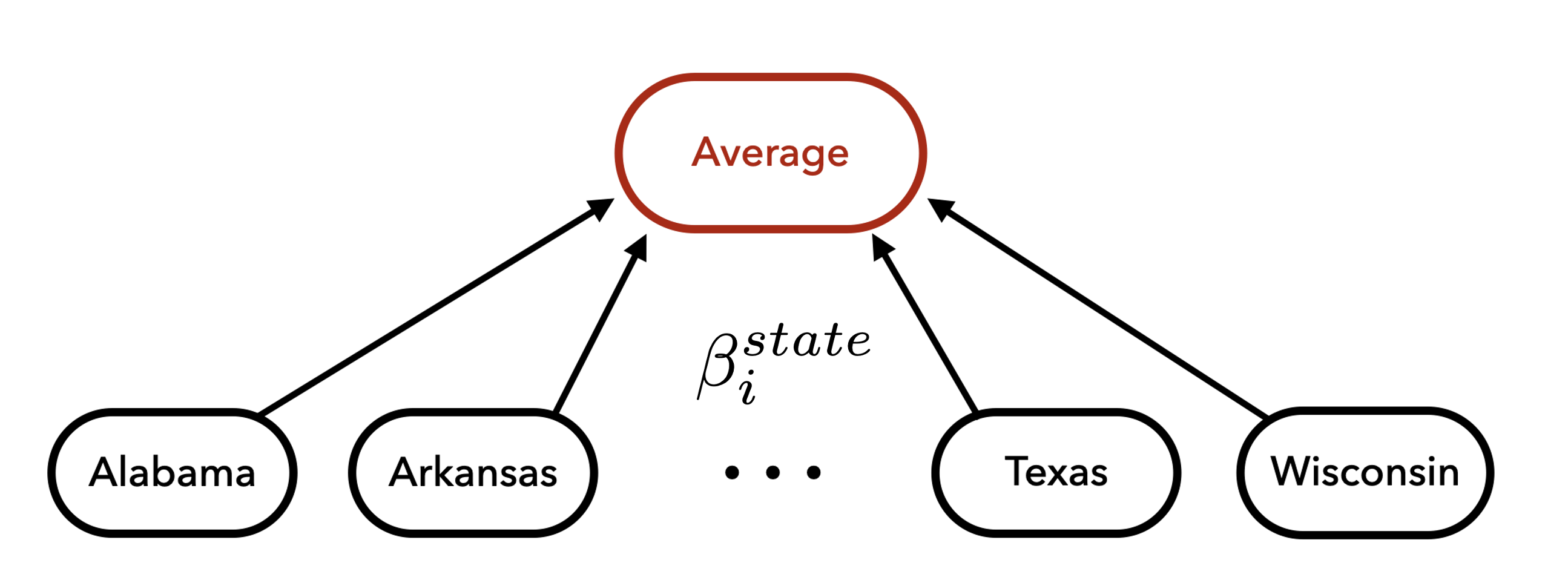
Shrinkage Across States

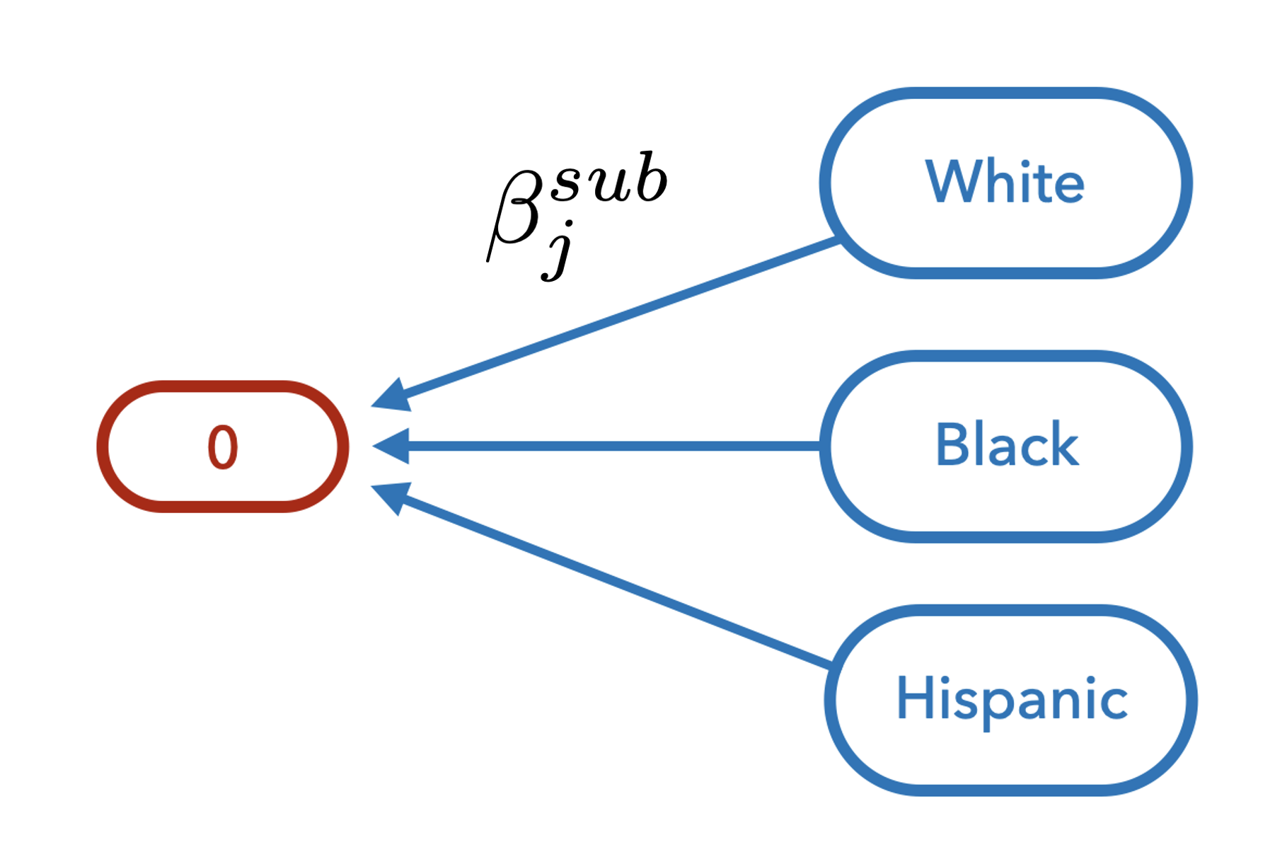
Shrinkage Across Subcategories

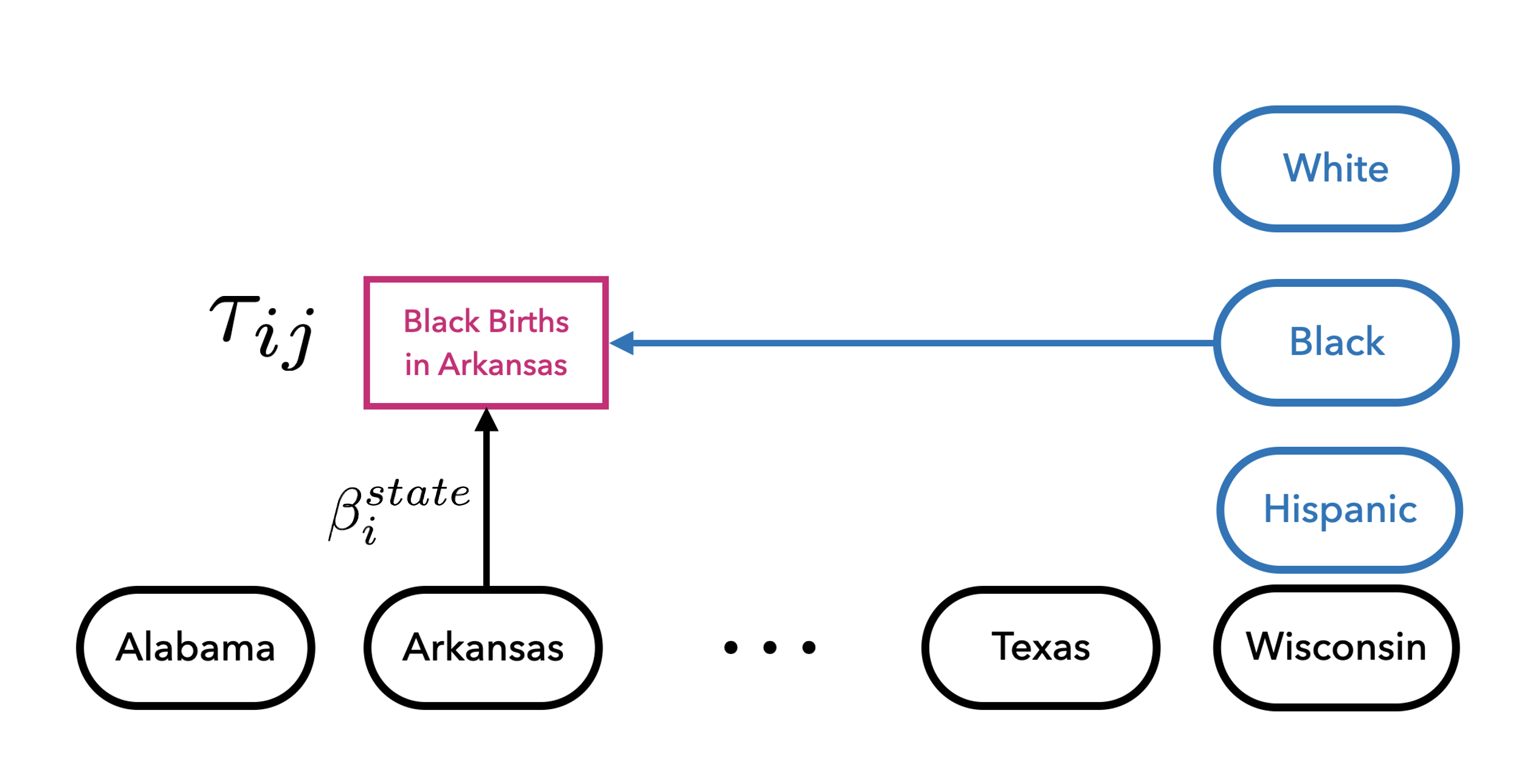
Variation Across Multiple Sources

MCMC Inference

• Model implemented in probabilistic programming library, numpyro

• MCMC inference with Hamiltonian Monte Carlo

• Run multiple chains, check Rhats and effective sample sizes

MCMC Inference

• Fit models for each category

  • Mortality: Total, race/ethnicity, timing of death and type of death
  • Fertility: Total, age, race/ethnicity, education, insurance

• For each, fit models for multiple latent ranks and check fit

• Code available at:

  • github.com/afranks86/dobbs_fertility
  • github.com/afranks86/dobbs_infant_mortality

Model Selection and Checking

• In-sample checks:
  • Question: how well does the model fit the observed data
  • Tool: gap plots and posterior predictive comparisons
  • Used to select latent factor rank
• Out-of-sample checks
  • Question: how well can we forecast
  • Tool: placebo-in-time checks

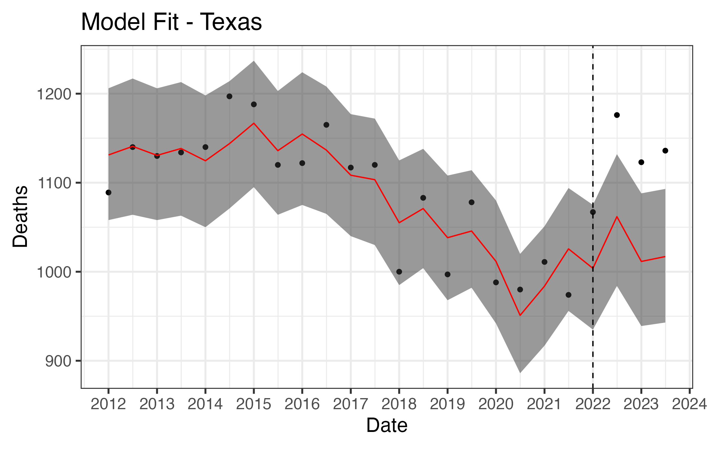
Results - Texas

Posterior Predictive Checks

• Posterior predictive checks are used to assess how well a Bayesian model fits observed data

• Unlike classical hypothesis testing, posterior predictive checks focus on practical significance of model inadequacies

• \(\mathbb{P}(T^{\text{pred}} > T^{\text{obs}} \mid Y) = \int \mathbb{P}(T^{\text{pred}} > T^{\text{obs}} \mid Y, \theta) \mathbb{P}(\theta \mid Y) d\theta\) should be far from 0 and 1.

Posterior Predictive Checks

• Maximum absolute residual: identify outliers inconsistent with the model: \(T_{ij} = \tau_{ij} = \max_{t} | r_{ijy}|\)

• Residual autocorrelation: check for remaining autocorrelation after controlling latent factors (and seasonal trends)

  • Test statistic based on residual autocorrelation at different lags
  • \(T_{ij} = cor(r_{ijt}, r_{i,j,t+l})\)

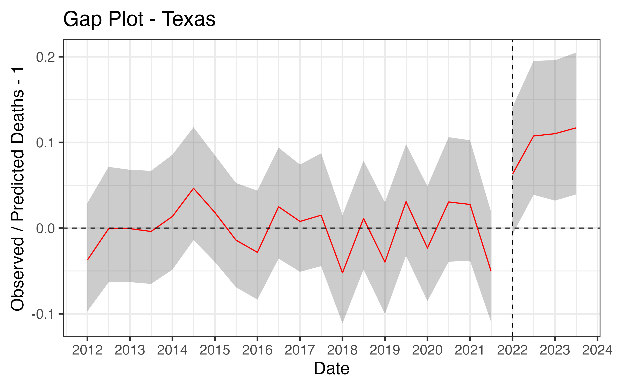
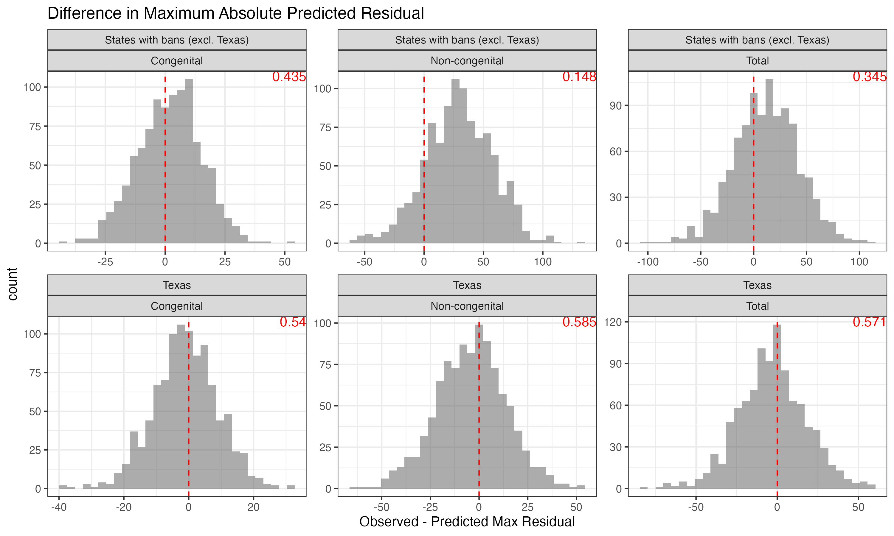
PPC: Max Residual

Posterior Predictive Checks

Across-unit correlation: states should be uncorrelated after controlling for latent factors:

• Test statistic based on eigenspectrum of residual correlation matrix

• Let \(\mathcal{C} = (c_{ii'})\) where \({c}_{ii'} =\) cor(\({r}_{i\cdot}, {r}_{i'\cdot}\))
• \(T = \sigma_{max}(\mathcal{C})\) where \(\sigma_{max}(\mathcal{C})\) is the largest singular of \(\mathcal{C}\).
• T should be small for uncorrelated state-residuals

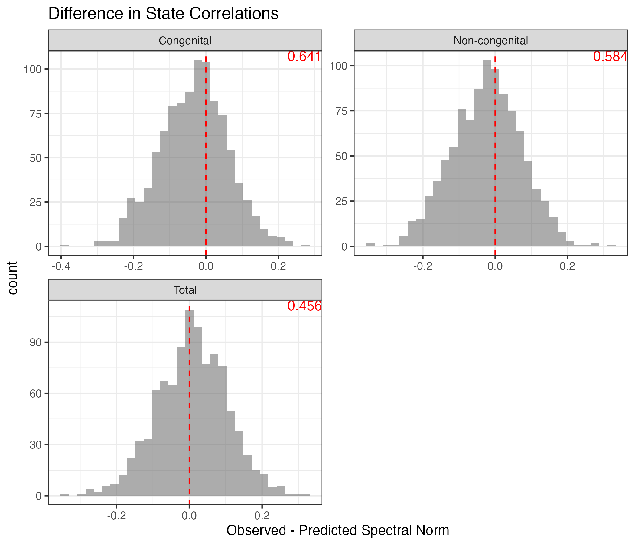
PPC: State Correlations

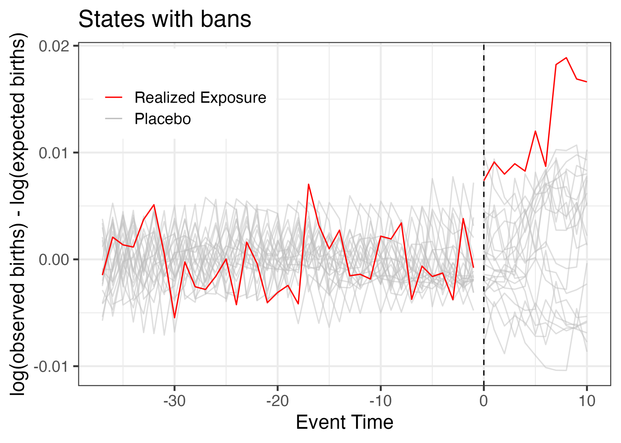
Placebo-in-Time

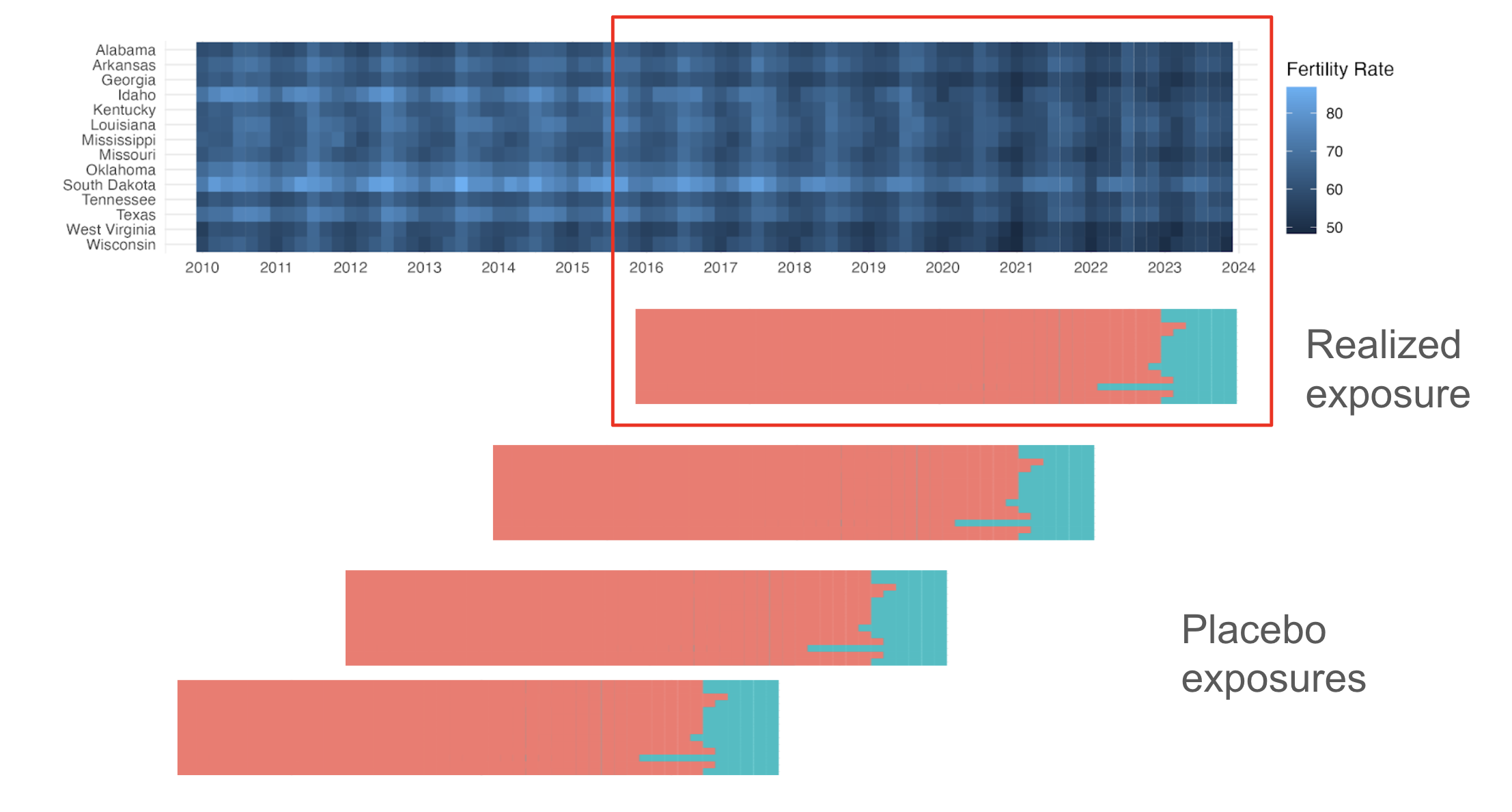
Placebo-in-Time

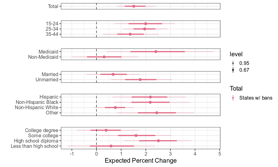
Fertility Impact by Subgroup

+1.7% overall increase

State-Specific Effects on Inf. Mortality

In banned states overall, the infant mortality rate increased by 5.6%

• Kentucky: +7.5%
• Texas: +8.9%

Effect on Infant Mortality by Cause

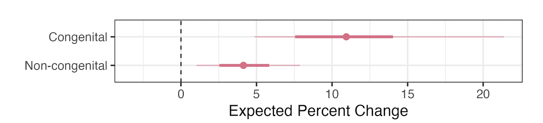
• +10.9% increase in congenital deaths
• +4.2% increase in non-congenital deaths

• Note: majority of deaths attributable to the bans are non-congenital

Effect on Infant Mortality by Race/Ethnicity

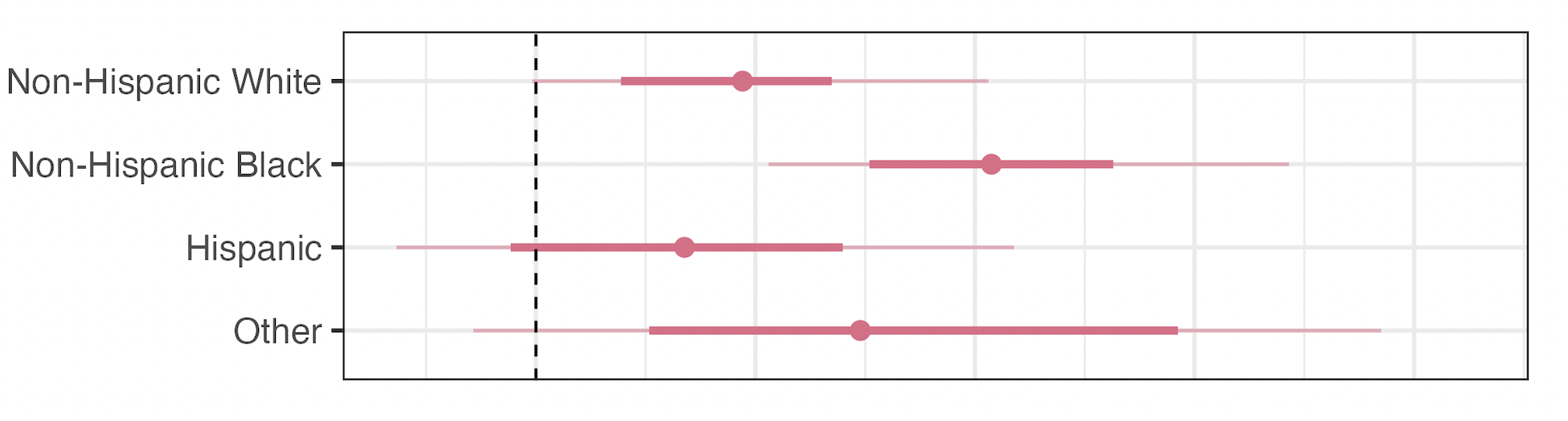
• NH White: +5.1%
• NH Black: +11.0%
• Hispanic: +3.3%
• NH Other: +9.9%

Key Findings

• Strong evidence that birth rates increased above expectation in states that banned abortion (+1.6%)

  • Slightly smaller than prior studies

  • Similar in magnitude of recent population-wide events

  • Largest impacts among those experiencing greatest structural disadvantage (consistent across states)

• Infant mortality increased in states with bans (+5.5%)
  • Outsized influence of Texas
  • Double the impact among non-Hispanic Black infants
  • Larger relative increase among congenital deaths

Implications

• Profound health, social and economic implications of being unable to obtain an abortion (Greene Foster 2020)
• State-specific policies and social contexts may present additional barriers for disadvantaged women
• Bans exacerbate existing health disparities
• Future work: impact of abortion bans on maternal morbidity, high-risk pregnancy care, and birth outcomes (e.g., preterm birth, low birthweight)

Methodological Takeaways

• Missing data and staggered adoption are easier to handle with Bayesian models

• Hierarchical modeling of the treatment effect in panel data is an underexplored strategy for estimating heterogeneous treatment effects

• Choice of temporal aggregation is important and tied to the amount of missingness

• More work needed to understand how and when to disaggregate when inferring total effects

Publications

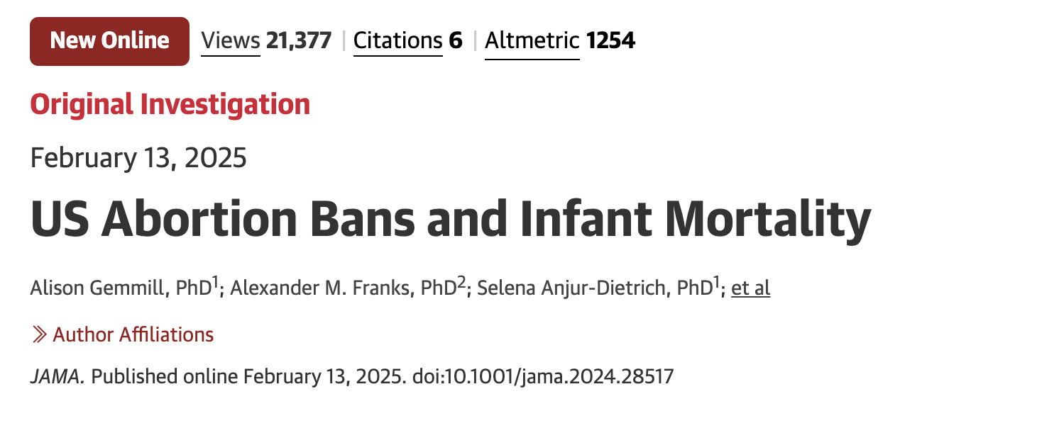
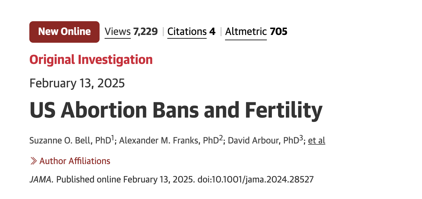
Papers published in JAMA. See Gemmill et al. (2025) and Bell et al. (2025). Supplementary materials contain modeling details.

Thank you!

Bell, Suzanne O, Alexander M Franks, David Arbour, Selena Anjur-Dietrich, Elizabeth A Stuart, Eli Ben-Michael, Avi Feller, and Alison Gemmill. 2025. “US Abortion Bans and Fertility.” JAMA.

Caraher, Raymond. 2024. “Do Abortion Bans Affect Reproductive and Infant Health? Evidence from Texas’s 2021 Ban and Its Impact on Health Disparities.” Political Economy Research Institute Working Paper No 606.

Dench, Daniel, Mayra Pineda-Torres, and Caitlin Myers. 2024. “The Effects of Post-Dobbs Abortion Bans on Fertility.” Journal of Public Economics 234: 105124.

Gemmill, Alison, Alexander M. Franks, Selena Anjur-Dietrich, Amy Ozinsky, David Arbour, Elizabeth A. Stuart, Eli Ben-Michael, Avi Feller, and Suzanne O. Bell. 2025. “US Abortion Bans and Infant Mortality.” JAMA 333 (15): 1315–23. https://doi.org/10.1001/jama.2024.28517.

Gemmill, Alison, Claire E Margerison, Elizabeth A Stuart, and Suzanne O Bell. 2024. “Infant Deaths After Texas’ 2021 Ban on Abortion in Early Pregnancy.” JAMA Pediatrics 178 (8): 784–91.

Sun, Liyang, Eli Ben-Michael, and Avi Feller. 2024. “Temporal Aggregation for the Synthetic Control Method.” In AEA Papers and Proceedings, 114:614–17. American Economic Association 2014 Broadway, Suite 305, Nashville, TN 37203.

Additional Slides

Fertility Data

• Bimonthly (e.g., January-February) counts of live births for 50 states and DC from birth certificates for 2014-2023
  • Compiled by the National Center for Health Statistics (NCHS)
  • 2023 provisional data

• Denominators (women 15-44) by state-year for 2014-2022 (imputed 2023)
  • Census: total counts and by age, race/ethnicity
  • American Community Survey: proportion by education, marital status, insurance (indirectly)

Fertility Approach

• Outcome: fertility rate (births per 1,000 per year)
• Exposure: 6-week or complete abortion ban (14 states¹), staggered adoption
• Pre-policy period: January 2014 through ~December 2022
• Treated period: ~January 2023 through December 2023

• Subgroups
  • Age: 15-24, 25-34, 35-44
  • Race/ethnicity: non-Hispanic White, non-Hispanic Black, Hispanic, and Other
  • Marital status: married, not married
  • Educational attainment: <high school, high school degree, some college, college degree+
  • Insurance payer for the delivery: Medicaid, non-Medicaid

1. States include Alabama, Arkansas, Georgia, Idaho, Kentucky, Louisiana, Mississippi, Missouri, Oklahoma, South Dakota, Tennessee, Texas, West Virginia, Wisconsin

Infant Mortality Data

• Biannual (e.g., January-June) counts of infant deaths (< 1 year) for 50 states and DC from death certificates for 2012-2023
  • 2023 provisional data
  • Impute suppressed data
• Denominators (live births) by state-biannual period for 2012-2023 from birth certificates

Missing Data

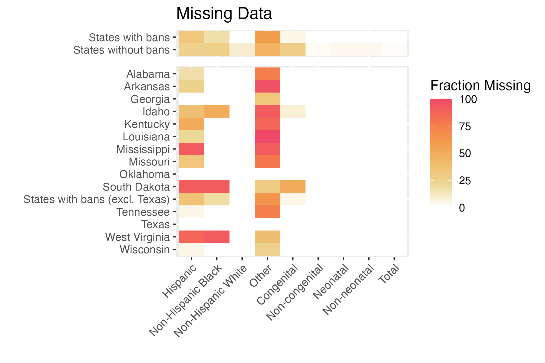
Note: missingness depends on level of temporal aggregation

Median Infant Deaths per Half-Year

State-Specific Effects on Fertility Rate

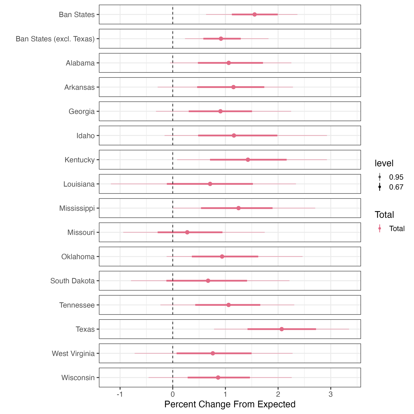
• Range: 0.6% - 2.1%

• Overall: +1.7%

• Non-Texas: +0.9%

Likelihood - Infant Mortality

Let \(M_{ijt}\) denote the indicator for suppressed counts, with \(M_{ijt}=1\) if \(0 < Y_{ijt}^{\text{obs}} < 10\) and \(M_{ijt}=0\) otherwise. % If we let \(B_{ijt}^{obs} = B_{ijt}(G_i)^{D_{ijt}}B_{ijt}(\infty)^{(1-D_{ijt})}\) then, The observed data likelihood can then be written as: \[\begin{align} \label{eq:obs_data_likelihood} \mathbb{P}(\mathbf{Y}^{obs}, \mathbf{M} \mid \mathbf{B}^{obs}, \mathbf{D}, \rho, \tau) =& \prod_{ijt}\left[ ((1-P_{\text{miss}}(\rho_{ijt}B_{ijt}^{obs}))\text{Pois}(Y_{ijt}; \rho_{ijt}B_{ijt}^{obs}))^{(1-M_{ijt})(1-D_{ijt})}\right. \times \\ &((1-P_{\text{miss}}(\tau_{ijt}\rho_{ijt}B_{ijt}^{obs}))~\text{Pois}(Y_{ijt}; \tau_{ijt}\rho_{ijt}B_{ijt}^{obs} ))^{{(1-M_{ijt})D_{ijt}}}\times \\ &\left.(P_{\text{miss}}(\rho_{ijt}B_{ijt}^{obs})^{M_{ijt}(1-D_{itj})}(P_{\text{miss}}(\tau_{ijt}\rho_{ijt}B_{ijt}^{obs})^{M_{ijt}D_{itj}})\right]. \end{align}\] where \(\text{Pois}(Y_{ijt}; \rho_{ijt}B_{ijt}^{obs})\) is the poisson PMF with mean \(\rho_{ijt}B_{ijt}^{obs}\) evaluated at \(Y_{ijt}\); and \[P_{\text{miss}}(\rho_{ijt}B_{ijt}^{obs}) = (F(9; \rho_{ijt}B_{ijt}^{obs}) - F(0; \rho_{ijt}B_{ijt}^{obs})), \] where \(F(a; \mu)\) is the CDF of a Poisson with mean \(\mu\) evaluated at \(a\) so that \(P_{\text{miss}}(\mu_{ijt}) = F(9; \mu) - F(0; \mu)\) is the probability of observing a missing count between 1 and 9, inclusive.